Single-cell projects now reach millions of cells. This scale improves statistical power and reveals rare biology. However, it also introduces real challenges. Memory limits slow data analysis. Runtimes stretch. Computationally demanding results can become hard to reproduce. This blog discusses how you can quickly and efficiently analyze large single-cell datasets while minimizing computational demands.
Jump to a section in this blog:
- Start with an end-to-end plan
- Quality control that keeps you honest
- Make large gene spaces manageable by optimizing HVGs
- Make big data small with sketching approaches
- Normalize in a way that scales
- Handle batch effects with prevention first
- Subset to go deeper where it matters
- Special case: very large, very sparse data
Start with an end-to-end plan
Plan for scale before the first cell is captured. Multiplex samples early and balance inputs across pools if you can. Match processing protocols as closely as possible. These choices reduce batch effects and simplify downstream work.
Keep the biology in focus. Write down the hypotheses you want to test and the decisions you need to make. Let those goals guide parameter choices, such as QC thresholds, the sample-size sketching approach, cluster resolution, and where to invest time and resources in more intensive analyses. Finally, lock your software. Use containerized R and Python environments so collaborators can rerun your workflow without surprises.
Watch our webinar on Analyzing Large-Scale Datasets
In this webinar, the Single Cell Discoveries Data Team presented practical solutions for working with large datasets.
Quality control that keeps you honest
Begin with a clean object. Inspect the number of detected genes per cell, the number of UMIs per cell, and the percentage of mitochondrial UMI counts; these are standard indicators of cell integrity and sequencing quality.
QC Tip: Also examine the percentage of ribosomal protein gene UMIs per cell. Ribosomal protein genes (often annotated as RPS and RPL families) encode ribosomal proteins rather than rRNA, yet they can dominate expression profiles in stressed or dying cells. High ribosomal gene content often indicates poor-quality cells, in which transcriptional diversity is lost, and housekeeping processes predominate.
Set cutoffs with biological context in mind. Median absolute deviation (MAD) may work well for many datasets, but highly heterogeneous data may require dynamic thresholds tailored to each cell population. Always consider tissue type and library chemistry when defining these rules.
Finally, document everything: thresholds, rationale, and the number of cells retained. This transparency ensures reproducibility and allows others to follow your QC decisions.
Make large gene spaces manageable by optimizing HVGs
When compute resources are limited, be deliberate about how many highly variable genes (HVGs) you carry forward during data analysis. Selecting HVGs is intended to concentrate the signal, not to retain every fluctuating feature. Using more HVGs than necessary increases memory usage and runtime with diminishing returns, especially for large datasets.
Start with a conservative set and only expand if key biological distinctions are lost. Run the most computationally demanding steps (dimensionality reduction, neighborhood graph construction, and clustering) on this reduced feature space. Validate the choice by checking whether known markers and significant populations remain separable and compare against a larger HVG set if possible. The goal is sufficiency, not maximality: enough genes to capture structure without overwhelming the computational budget.
Make big data small with sketching approaches
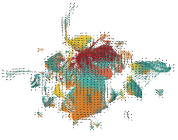
Random down-sampling is fast, but it risks discarding rare populations. In contrast, sketching approaches aim to select a representative subset that preserves heterogeneity. Create a sketch of about 25-50k cells from the full object. Run the heavier steps on this sketch. That includes clustering and marker-based annotation. Then project labels back to the full dataset for high-resolution plots and statistics.
Validate the sketch. Compare it to a size-matched random subset and overlay known markers. The sketch should retain signals that random sampling weakens. Be aware that some analysis tools may change the type or structure of your single-cell dataset. If you rely on reference-based annotation tools, confirm compatibility or stick to marker-driven labelling on the sketch.

A sketched subset captures the same biological structure as the full dataset, enabling faster clustering and annotation without losing heterogeneity.
Normalize in a way that scales
Choose normalization that respects depth while still running quickly. Log-normalization may seem quick and easy at first, but it under-corrects depth effects. SCT helps in some settings, especially for integration, but it can be slow and memory-intensive with very large objects. scran provides robust, depth-aware scaling and performs well at size when paired with a first-pass sketching.
A practical sequence looks like this:
- Create a sketch using the raw counts (remember, this is pre-normalization)
- Cluster it (for example, via scran’s quickCluster function)
- Project the quick clusters onto the full dataset
- Apply scran normalization to the full dataset using those approximated clusters
- Proceed with your analysis as usual, don’t forget to recompute your clusters using your normalized data!
Handle batch effects with prevention first
Good design is the best defence. Multiplex early, process together, and balance inputs. If batches still dominate your embedding, apply correction. Harmony aligns overlapping populations quickly. fastMNN is well-suited to many-to-many batch relationships in R pipelines. scVI handles complex designs and scales in Python. After correction, recheck marker recovery and differential abundance. If biology looks washed out, tune parameters or roll back.
Subset to go deeper where it matters
Once you have broad annotations, focuson a population or lineage of interest. Subsetting improves resolution, clarifies markers, and keeps compute costs under control. It also sets the stage for dynamic analyses.
Case Study: RNA Velocity adds trajectory and timing, but full-dataset runs can be highly computationally demanding and become a significant bottleneck. Focus on the subset that answers your question. Quantify gene-specific spliced and unspliced reads for selected clusters. Compute velocity and latent time on that subset. Integrate the results with your labels to describe cell-type-specific transitions and pathway shifts. You gain insight into dynamics without multi-day runs.
Special case: very large, very sparse data
Ultra-sparse, large matrices, such as those often encountered in sequencing-based spatial data, need extra care. Sketching can carry low-information data points forward. Increase the number of highly variable genes and verify that they align with the expected biology. Use a larger sketch to buffer sparsity. Confirm that the rare structure is preserved by comparing marker patterns and neighborhood composition between the sketch and the full object.
Avoid common pitfalls
- Environment drift is a frequent source of confusion. Containerize your analysis environment and record image digests/hashes alongside results.
- Break the workflow into small notebooks for QC, sketching, labeling, and velocity.
- Cache intermediate objects to avoid repeated work.
- Some sketching tools modify object classes. Confirm compatibility before running reference-based tools.
- Integration can also over-correct. If known biology fades, reduce correction strength or change the method.
Key takeaways
Begin with a comprehensive, end-to-end plan that keeps the biological questions at the center. Use sketching to keep analyses fast and protect rare biology. Reduce the complexity of your dataset when possible. Focus on advanced methods on subsets that answer your question. Containerize the environment so the entire workflow remains easy to reproduce.
Partner with our data team
If you run your project with Single Cell Discoveries, our data analysis team reviews every dataset and delivers an exploratory report. We sanity-check data quality, establish an initial set of key parameters, and share clear first-pass results, such as cleaned count tables, low-dimensional embeddings, and early differential gene-expression patterns. You start from a well-documented object and a concise report that helps you validate design choices and decide on the next steps.
If you want to go further, our data consulting team can help with custom analyses and special requests. We work with you to extend the exploratory report into targeted hypothesis tests, tailored models, cross-study integrations, and publication-ready figures.
In short, every project includes analysis and an exploratory report. When you need deeper insights or specialized workflows, you can partner with our consulting team to get the results you need.